Linear regression is one of the simplest and most widely used techniques in data science. If you’ve ever wondered how we can predict future values based on existing data, linear regression is a great place to start!

In this blog, we’ll explain linear regression in simple terms, go through its mathematical intuition, and show how to implement it with Python code. By the end, even a non-tech person will have a good grasp of this concept.

What is Linear Regression?

Imagine you’re trying to predict how much you’ll spend on groceries based on the number of items in your cart. You might notice that the more items you add, the higher your bill becomes. If you were to plot the number of items on the x-axis and the total cost on the y-axis, you might see a pattern: a straight line can roughly describe the relationship.

Linear regression is a method that tries to find the best straight line that fits such data. This line can then be used to predict future values.

The Goal of Linear Regression

The main goal of linear regression is to find the line of best fit, which minimizes the difference between the actual data points and the predicted values given by the line.

Why and When is Linear Regression Required?

Linear regression is required when we want to establish a relationship between two variables and make predictions. It works well when:

1. There is a linear relationship between variables: Linear regression is suitable when the data shows a roughly straight-line relationship.

2. You want to predict a continuous output: For example, predicting house prices, sales revenue, or the temperature based on some independent factors.

3. You want an interpretable model: Since the output is based on a simple equation y = mx + c, it’s easy to understand how changes in the input affect the output.

4. You need a baseline model: Linear regression is often used as a baseline model in machine learning to compare against more complex algorithms.

Mathematical Intuition Behind Linear Regression

The equation of a straight line is:

y = mx + c

Where:

– y is the predicted value (dependent variable)

– x is the input value (independent variable)

– m is the slope of the line (how steep the line is)

– c is the y-intercept (where the line crosses the y-axis)

Visualizing the Line of Best Fit

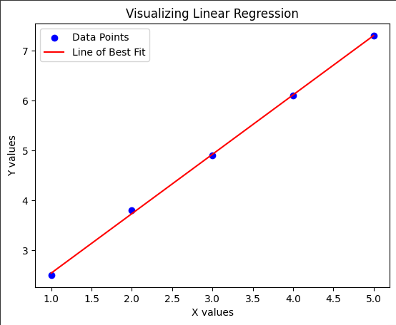
Below is a simple visualization of a dataset and a line of best fit.

This graph shows how the red line (line of best fit) closely follows the trend of the blue data points.

Finding the Best Line

In linear regression, our goal is to find the values of m and c that give us the line closest to our data points. The way we measure how close the line is to the actual data is by using a metric called the mean squared error (MSE).

The formula for MSE is:

Where:

• N is the number of data points
• yᵢ is the actual value of the i-th data point
• ŷᵢ is the predicted value from our line for the i-th data point

We want to minimize this error by adjusting m and c. This is typically done using a technique called gradient descent, which iteratively improves the values of m and c until the error is as small as possible.

Python Implementation of Linear Regression

Now that we understand the basics, let’s see how we can implement linear regression in Python.

Example: Predicting House Prices Based on Area

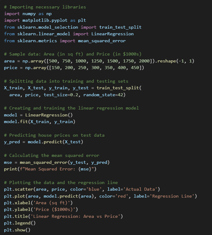
Let’s assume we have some data on house prices and their corresponding areas. We’ll use this data to build a simple linear regression model.

Explanation:

1. Data Preparation: We start by defining our input (area) and output (price) data.
2. Train-Test Split: We split the data into training and testing sets to evaluate the model’s performance.
3. Model Creation: We create an instance of the Linear Regression class and train it using the fit method.
4. Prediction: We use the trained model to predict house prices on the test data.
5. Error Calculation: We calculate the mean squared error to measure how well our model performed.
6. Visualization: Finally, we plot the data and the regression line to visualize the relationship.

Interpreting the Results

The red line in the plot represents the line of best fit. As you can see, it closely follows the trend of the data points. This means our model has successfully captured the relationship between area and price.

If the mean squared error is small, it indicates that the model’s predictions are close to the actual values.

Key Takeaways

1. Linear regression is simple but powerful: Despite its simplicity, linear regression is a fundamental technique in data science and machine learning.

2. Mathematics matters: Understanding the math behind the model helps us know how it works and when to use it.

3. Code implementation is straightforward: With libraries like `scikit-learn`, implementing linear regression in Python is quick and easy.

Conclusion

Linear regression is a great starting point for anyone interested in data science and machine learning. It’s easy to understand, implement, and interpret. By learning how to use it, you’re taking your first steps toward building more complex models.