Introduction: The Journey From Data to Insights

In today’s data-driven world, the ability to transform raw data into actionable insights is nothing short of a superpower. However, the path from messy data to valuable business outcomes is rarely straightforward. As a data science expert with over a decade of experience, I’ve witnessed firsthand how a structured workflow can make all the difference between project success and failure.

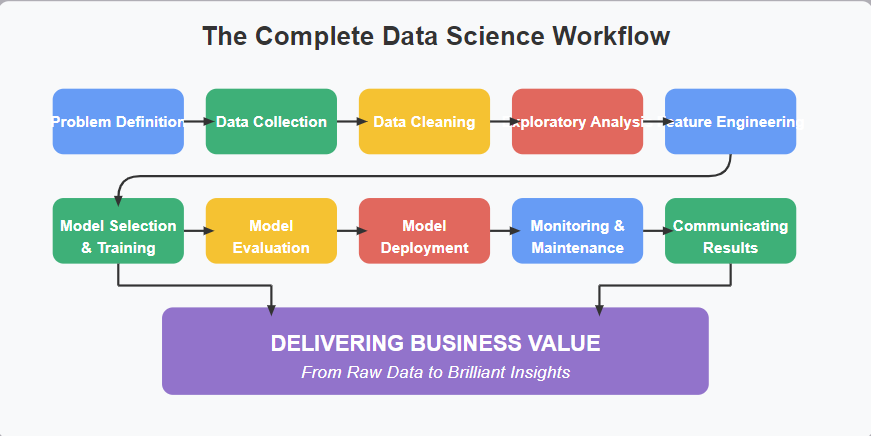
The data science workflow is essentially a roadmap that guides you through the entire process. Without a clear workflow, you might find yourself lost in endless data cleaning or creating models that don’t actually solve business problems. Therefore, understanding each step in this journey is crucial for anyone looking to harness the power of data.

In this comprehensive guide, we’ll explore the complete data science workflow, from initial problem definition to final deployment and monitoring. Moreover, we’ll dive into practical tips and real-world examples that will help you navigate this exciting but complex field.

Problem Definition: Starting With the Right Questions

Every successful data science project begins with a clear problem definition. In fact, this first step is often the most critical yet overlooked part of the entire workflow.

Start by asking fundamental questions: What business problem are we trying to solve? What decisions will be made based on our insights? Who are the stakeholders, and what do they need? Furthermore, establishing clear success metrics upfront will help you measure progress and demonstrate value.

Here’s a simple framework to guide your problem definition:

1. Business Objective: Define the specific business goal you’re trying to achieve.
2. Success Criteria: Establish measurable outcomes that indicate success.
3. Constraints: Identify any limitations such as time, budget, or data availability.
4. Stakeholders: List all parties who will use or be affected by the results.
5. Value Proposition: Clearly articulate how solving this problem creates value.

Remember, a well-defined problem is already half-solved. Hence, invest sufficient time in this crucial first step.

Data Collection: Gathering the Right Information in Data Science

Once you’ve clearly defined the problem, the next step is to collect relevant data. However, this process involves more than just downloading datasets or querying databases.

First, identify all potential data sources, both internal and external. Then, assess the quality, relevance, and accessibility of each source. Additionally, consider privacy regulations and ethical considerations that might impact your data collection process.

Common data collection methods include:

• Database Queries: Extracting data from relational databases using SQL
• APIs: Accessing data from web services and applications
• Web Scraping: Collecting data from websites (when legal and ethical)
• Surveys and Forms: Gathering primary data directly from users
• IoT Devices: Collecting sensor data from connected devices

For example, if you’re working on a customer churn prediction project, you might need to collect:

# Example: Collecting customer data from a database
import pandas as pd
from sqlalchemy import create_engine

# Connect to the database
engine = create_engine('postgresql://username:password@hostname/database')

# Query to collect customer data
query = """
SELECT 
    customer_id,
    signup_date,
    last_purchase_date,
    total_purchases,
    avg_order_value,
    support_tickets_count,
    subscription_plan,
    is_churned
FROM customers
LEFT JOIN transactions USING (customer_id)
WHERE signup_date >= '2023-01-01'
"""

# Load the data into a pandas DataFrame
customer_data = pd.read_sql(query, engine)

Remember, the quality of your insights can never exceed the quality of your data. Therefore, be thorough and strategic in your data collection efforts.

Data Cleaning: Preparing for Analysis in Data Science

Raw data is rarely ready for analysis. Instead, it often contains errors, missing values, and inconsistencies that need to be addressed before moving forward.

Data cleaning is typically the most time-consuming phase of the data science workflow. Nevertheless, it’s absolutely essential for reliable results. Here are key steps in the data cleaning process:

1. Handling Missing Values: Decide whether to impute missing data or remove incomplete records.
2. Removing Duplicates: Identify and eliminate redundant data points.
3. Fixing Data Types: Ensure each column has the appropriate data type.
4. Standardizing Formats: Convert inconsistent formats (dates, currencies, etc.) to a standard form.
5. Handling Outliers: Identify and address extreme values that might skew your analysis.

Let’s look at a practical example of data cleaning:

# Example: Data cleaning for customer churn analysis
import pandas as pd
import numpy as np

# Load the dataset
df = customer_data.copy()

# Check for missing values
print(f"Missing values per column:n{df.isnull().sum()}")

# Handle missing values
# For numeric columns, fill with median
numeric_cols = df.select_dtypes(include=[np.number]).columns
df[numeric_cols] = df[numeric_cols].fillna(df[numeric_cols].median())

# For categorical columns, fill with mode
cat_cols = df.select_dtypes(include=['object']).columns
for col in cat_cols:
    df[col] = df[col].fillna(df[col].mode()[0])

# Convert date columns to datetime
df['signup_date'] = pd.to_datetime(df['signup_date'])
df['last_purchase_date'] = pd.to_datetime(df['last_purchase_date'])

# Create a new feature: customer tenure in days
df['tenure_days'] = (df['last_purchase_date'] - df['signup_date']).dt.days

# Remove outliers (example: customers with unrealistic purchase amounts)
df = df[df['avg_order_value'] < df['avg_order_value'].quantile(0.99)]

# Check the clean dataset
print(f"Dataset shape after cleaning: {df.shape}")

Remember, thorough data cleaning might not be glamorous, but it’s the foundation of trustworthy analysis. Consequently, allocate sufficient time and attention to this critical step.

Exploratory Data Analysis (EDA): Understanding Your Data in Data Science

After cleaning your data, it’s time to explore and understand it better. Exploratory Data Analysis (EDA) helps you discover patterns, spot anomalies, and generate hypotheses about your data.

During EDA, you’ll examine distributions, correlations, and relationships between variables. Furthermore, you’ll visualize your data to gain insights that might not be apparent from raw numbers.

Key techniques in EDA include:

1. Descriptive Statistics: Calculate means, medians, standard deviations, etc.
2. Distribution Analysis: Examine how values are distributed across your dataset.
3. Correlation Analysis: Identify relationships between different variables.
4. Temporal Analysis: Look for trends or patterns over time.
5. Segmentation: Analyze how metrics differ across different segments.

Here’s an example of EDA for our customer churn analysis:

# Example: EDA for customer churn analysis
import pandas as pd
import matplotlib.pyplot as plt
import seaborn as sns

# Set the style for the visualizations
sns.set(style="whitegrid")

# Basic descriptive statistics
print(df.describe())

# Visualize churn rate
plt.figure(figsize=(10, 6))
churn_rate = df['is_churned'].mean() * 100
plt.bar(['Retained', 'Churned'], [100 - churn_rate, churn_rate])
plt.title('Customer Churn Rate')
plt.ylabel('Percentage (%)')
plt.show()

# Analyze churn by subscription plan
plt.figure(figsize=(12, 6))
sns.countplot(x='subscription_plan', hue='is_churned', data=df)
plt.title('Churn by Subscription Plan')
plt.xlabel('Subscription Plan')
plt.ylabel('Count')
plt.show()

# Correlation analysis
plt.figure(figsize=(12, 10))
correlation = df.select_dtypes(include=[np.number]).corr()
mask = np.triu(correlation)
sns.heatmap(correlation, annot=True, mask=mask, cmap='coolwarm')
plt.title('Correlation Matrix')
plt.show()

Through EDA, you’ll gain valuable insights that will inform your feature engineering and modeling decisions. Additionally, you’ll be able to communicate initial findings to stakeholders early in the project.

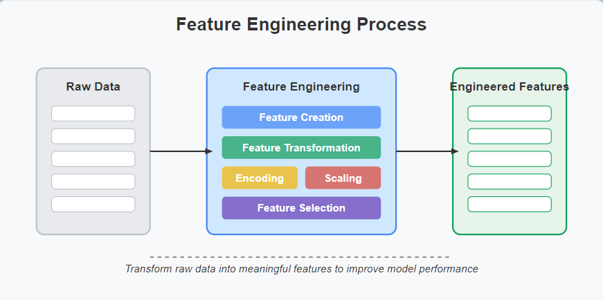
Feature Engineering: Creating Meaningful Variables in Data Science

Feature engineering is the process of transforming raw data into features that better represent the underlying problem, resulting in improved model performance.

This step involves creating new variables, transforming existing ones, and selecting the most relevant features for your model. Moreover, it’s where domain expertise becomes particularly valuable.

Common feature engineering techniques include:

1. Feature Creation: Generating new variables based on existing ones.
2. Feature Transformation: Applying mathematical functions to improve feature distribution.
3. Encoding: Converting categorical variables into numerical representations.
4. Dimensionality Reduction: Reducing the number of features while preserving information.
5. Feature Scaling: Normalizing or standardizing features to a common scale.

Here’s an example of feature engineering for our churn prediction model:

# Example: Feature engineering for churn prediction
import pandas as pd
from sklearn.preprocessing import StandardScaler, OneHotEncoder
from sklearn.compose import ColumnTransformer
from sklearn.pipeline import Pipeline

# Define numeric and categorical features
numeric_features = ['tenure_days', 'total_purchases', 'avg_order_value', 'support_tickets_count']
categorical_features = ['subscription_plan']

# Create a preprocessing pipeline
preprocessor = ColumnTransformer(
    transformers=[
        ('num', StandardScaler(), numeric_features),
        ('cat', OneHotEncoder(), categorical_features)
    ])

# Create new features
df['recency'] = (pd.Timestamp.now() - df['last_purchase_date']).dt.days
df['purchase_frequency'] = df['total_purchases'] / df['tenure_days']
df['support_ticket_rate'] = df['support_tickets_count'] / df['tenure_days']

# Apply preprocessing
X = df.drop('is_churned', axis=1)
y = df['is_churned']

# Create a pipeline with preprocessing
pipeline = Pipeline(steps=[('preprocessor', preprocessor)])
X_processed = pipeline.fit_transform(X)

print(f"Shape after feature engineering: {X_processed.shape}")

Well-engineered features can significantly improve model performance. Therefore, invest time in this creative process, combining your domain knowledge with data insights.

Model Selection and Training: Finding the Right Approach in Data Science

Now that your data is prepared and your features are engineered, it’s time to select and train a model. This step involves choosing the right algorithm and fine-tuning its parameters.

The model selection depends on your problem type (classification, regression, clustering, etc.) and specific requirements like interpretability, speed, and accuracy. Additionally, you’ll need to decide on a suitable evaluation metric.

Here’s a process for model selection and training:

1. Split the Data: Divide your dataset into training, validation, and test sets.
2. Baseline Model: Establish a simple baseline model for comparison.
3. Model Selection: Try different algorithms suitable for your problem.
4. Hyperparameter Tuning: Optimize model parameters for better performance.
5. Evaluation: Assess model performance using appropriate metrics.

Let’s implement this process for our churn prediction example:

# Example: Model selection and training for churn prediction
from sklearn.model_selection import train_test_split, GridSearchCV
from sklearn.ensemble import RandomForestClassifier, GradientBoostingClassifier
from sklearn.linear_model import LogisticRegression
from sklearn.metrics import accuracy_score, precision_score, recall_score, f1_score, roc_auc_score

# Split the data
X_train, X_test, y_train, y_test = train_test_split(X_processed, y, test_size=0.2, random_state=42)

# Define models to try
models = {
    'Logistic Regression': LogisticRegression(max_iter=1000),
    'Random Forest': RandomForestClassifier(),
    'Gradient Boosting': GradientBoostingClassifier()
}

# Train and evaluate each model
results = {}
for name, model in models.items():
    model.fit(X_train, y_train)
    y_pred = model.predict(X_test)
    
    # Calculate metrics
    results[name] = {
        'accuracy': accuracy_score(y_test, y_pred),
        'precision': precision_score(y_test, y_pred),
        'recall': recall_score(y_test, y_pred),
        'f1': f1_score(y_test, y_pred),
        'roc_auc': roc_auc_score(y_test, model.predict_proba(X_test)[:, 1])
    }

# Print results
for model, metrics in results.items():
    print(f"n{model}:")
    for metric, value in metrics.items():
        print(f"  {metric}: {value:.4f}")

# Select the best model (based on F1 score in this example)
best_model_name = max(results, key=lambda x: results[x]['f1'])
print(f"nBest model: {best_model_name}")

# Fine-tune the best model (example for Random Forest)
if best_model_name == 'Random Forest':
    param_grid = {
        'n_estimators': [100, 200, 300],
        'max_depth': [None, 10, 20, 30],
        'min_samples_split': [2, 5, 10]
    }
    
    grid_search = GridSearchCV(RandomForestClassifier(), param_grid, cv=5, scoring='f1')
    grid_search.fit(X_train, y_train)
    
    print(f"Best parameters: {grid_search.best_params_}")
    print(f"Best score: {grid_search.best_score_:.4f}")
    
    # Update the best model
    best_model = grid_search.best_estimator_
else:
    best_model = models[best_model_name]

Remember, the goal is not just to achieve the highest accuracy but to build a model that solves the business problem effectively. Therefore, consider factors like interpretability, deployment constraints, and long-term maintenance.

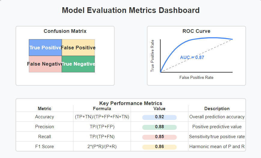
Model Evaluation: Assessing Performance and Impact

After training your model, it’s crucial to evaluate it thoroughly to ensure it meets your requirements. This evaluation should go beyond basic metrics to include business impact assessment.

Consider these aspects when evaluating your model:

1. Technical Metrics: Accuracy, precision, recall, F1-score, etc.
2. Business Metrics: Return on investment, cost savings, revenue increase, etc.
3. Interpretability: How well can the model’s decisions be explained?
4. Fairness: Does the model perform equally well across different segments?
5. Robustness: How well does the model handle edge cases and outliers?

Here’s how you might evaluate your churn prediction model:

# Example: Comprehensive model evaluation for churn prediction
from sklearn.metrics import confusion_matrix, classification_report, roc_curve
import matplotlib.pyplot as plt
import seaborn as sns

# Get predictions from the best model
y_pred = best_model.predict(X_test)
y_prob = best_model.predict_proba(X_test)[:, 1]

# Confusion matrix
plt.figure(figsize=(8, 6))
cm = confusion_matrix(y_test, y_pred)
sns.heatmap(cm, annot=True, fmt='d', cmap='Blues')
plt.xlabel('Predicted')
plt.ylabel('Actual')
plt.title('Confusion Matrix')
plt.show()

# Classification report
print("nClassification Report:")
print(classification_report(y_test, y_pred))

# ROC curve
plt.figure(figsize=(8, 6))
fpr, tpr, _ = roc_curve(y_test, y_prob)
plt.plot(fpr, tpr, label=f'AUC = {roc_auc_score(y_test, y_prob):.4f}')
plt.plot([0, 1], [0, 1], 'k--')
plt.xlabel('False Positive Rate')
plt.ylabel('True Positive Rate')
plt.title('ROC Curve')
plt.legend()
plt.show()

# Feature importance (for interpretability)
if hasattr(best_model, 'feature_importances_'):
    plt.figure(figsize=(10, 8))
    
    # Get feature names
    numeric_features_list = numeric_features + ['recency', 'purchase_frequency', 'support_ticket_rate']
    ohe = preprocessor.named_transformers_['cat']
    categorical_features_list = list(ohe.get_feature_names_out(categorical_features))
    feature_names = numeric_features_list + categorical_features_list
    
    # Plot feature importance
    feature_importance = pd.DataFrame({
        'feature': feature_names[:len(best_model.feature_importances_)],
        'importance': best_model.feature_importances_
    }).sort_values('importance', ascending=False)
    
    sns.barplot(x='importance', y='feature', data=feature_importance)
    plt.title('Feature Importance')
    plt.show()

# Business impact assessment
# (This is a simplified example; actual analysis would depend on business specifics)
avg_customer_value = 500  # Assumed average customer lifetime value
retention_cost = 50  # Assumed cost to retain a customer
churn_rate = y_test.mean()

# Calculate potential savings
potential_churners = sum(y_prob > 0.5)
correct_predictions = sum((y_prob > 0.5) & (y_test == 1))
retention_success_rate = 0.3  # Assumption: 30% of retention efforts succeed

potential_savings = (correct_predictions * retention_success_rate * avg_customer_value) - (potential_churners * retention_cost)

print(f"nBusiness Impact Assessment:")
print(f"Potential annual savings: ${potential_savings:.2f}")
print(f"ROI: {(potential_savings / (potential_churners * retention_cost)):.2f}x")

A comprehensive evaluation helps you understand the model’s strengths and limitations. Furthermore, it allows you to communicate the expected business impact to stakeholders.

Model Deployment: Putting Insights into Action

Once you’ve developed a model that meets your requirements, it’s time to deploy it in a production environment. This step transforms your analytical work into a system that delivers actual business value.

Deployment can take many forms, from integrating with existing systems to creating new applications. Regardless of the approach, consider these aspects:

1. Scalability: Can the system handle the expected load?
2. Reliability: How robust is the system against failures?
3. Maintainability: How easy is it to update and improve the model?
4. Security: How is sensitive data protected?
5. Usability: How will end-users interact with the system?

Here’s a simplified example of model deployment using Flask:

# Example: Simple Flask API for churn prediction model
from flask import Flask, request, jsonify
import joblib
import pandas as pd

# Load the model and preprocessor
model = joblib.load('churn_model.pkl')
preprocessor = joblib.load('preprocessor.pkl')

app = Flask(__name__)

@app.route('/predict', methods=['POST'])
def predict():
    # Get data from request
    data = request.json
    
    # Convert to DataFrame
    df = pd.DataFrame([data])
    
    # Preprocess the data
    df['signup_date'] = pd.to_datetime(df['signup_date'])
    df['last_purchase_date'] = pd.to_datetime(df['last_purchase_date'])
    df['tenure_days'] = (df['last_purchase_date'] - df['signup_date']).dt.days
    df['recency'] = (pd.Timestamp.now() - df['last_purchase_date']).dt.days
    df['purchase_frequency'] = df['total_purchases'] / df['tenure_days']
    df['support_ticket_rate'] = df['support_tickets_count'] / df['tenure_days']
    
    # Transform using preprocessor
    X = preprocessor.transform(df)
    
    # Make prediction
    churn_probability = model.predict_proba(X)[0, 1]
    churn_prediction = bool(churn_probability > 0.5)
    
    # Return prediction
    return jsonify({
        'customer_id': data['customer_id'],
        'churn_probability': float(churn_probability),
        'churn_prediction': churn_prediction,
        'recommended_action': 'Retention offer' if churn_prediction else 'Standard service'
    })

if __name__ == '__main__':
    app.run(debug=True)

In addition to the technical aspects, consider how the model outputs will be used by stakeholders. Moreover, develop clear documentation and training to ensure proper use of the system.

Monitoring and Maintenance: Ensuring Long-term Success

Deploying a model is not the end of the journey. Data science projects require ongoing monitoring and maintenance to ensure continued performance and relevance.

As data distributions change over time (a phenomenon known as concept drift), your model’s performance may degrade. Additionally, business requirements may evolve, necessitating updates to your solution.

Key aspects of monitoring and maintenance include:

1. Performance Tracking: Monitor key metrics over time.
2. Data Quality Checks: Ensure incoming data remains consistent with training data.
3. Model Retraining: Update the model periodically with new data.
4. Version Control: Manage changes to models and code.
5. Documentation: Maintain clear documentation of the entire system.

Here’s a simple example of a monitoring script:

# Example: Simple monitoring script for a churn prediction model
import pandas as pd
import numpy as np
from sklearn.metrics import roc_auc_score, precision_score, recall_score
import matplotlib.pyplot as plt
import joblib
import datetime

# Load the model
model = joblib.load('churn_model.pkl')
preprocessor = joblib.load('preprocessor.pkl')

def evaluate_model_performance(data_path):
    """Evaluate model performance on new data."""
    # Load new data
    df = pd.read_csv(data_path)
    
    # Preprocess
    # (Same preprocessing steps as in deployment)
    
    # Get features and target
    X = preprocessor.transform(df.drop('is_churned', axis=1))
    y = df['is_churned']
    
    # Make predictions
    y_prob = model.predict_proba(X)[:, 1]
    y_pred = y_prob > 0.5
    
    # Calculate metrics
    auc = roc_auc_score(y, y_prob)
    precision = precision_score(y, y_pred)
    recall = recall_score(y, y_pred)
    
    # Log results
    log_entry = {
        'date': datetime.datetime.now().strftime('%Y-%m-%d'),
        'auc': auc,
        'precision': precision,
        'recall': recall,
        'data_size': len(df)
    }
    
    # Append to log
    try:
        log = pd.read_csv('model_performance_log.csv')
        log = log.append(log_entry, ignore_index=True)
    except:
        log = pd.DataFrame([log_entry])
    
    log.to_csv('model_performance_log.csv', index=False)
    
    # Plot performance over time
    plt.figure(figsize=(12, 6))
    plt.plot(log['date'], log['auc'], label='AUC')
    plt.plot(log['date'], log['precision'], label='Precision')
    plt.plot(log['date'], log['recall'], label='Recall')
    plt.xlabel('Date')
    plt.ylabel('Score')
    plt.title('Model Performance Over Time')
    plt.legend()
    plt.savefig('performance_trend.png')
    
    # Check for significant performance drop
    if len(log) > 1:
        auc_drop = log['auc'].iloc[-2] - log['auc'].iloc[-1]
        if auc_drop > 0.05:  # 5% drop in AUC
            print("WARNING: Significant performance drop detected!")
            print(f"AUC dropped by {auc_drop:.2%}")
            print("Consider retraining the model with recent data.")
    
    return log_entry

# Run evaluation monthly
if __name__ == '__main__':
    evaluate_model_performance('new_customer_data.csv')

Regular monitoring and maintenance ensure your data science solution continues to deliver value over time. Therefore, establish clear processes for these activities from the beginning.

Communicating Results: Sharing Insights Effectively

Throughout the data science workflow, effective communication is essential. This involves translating technical findings into language that stakeholders can understand and act upon.

Key aspects of communicating results include:

1. Audience Awareness: Tailor your message to your audience’s technical background and interests.
2. Visualization: Use charts and graphs to illustrate key points.
3. Storytelling: Frame your findings as a coherent narrative.
4. Actionability: Emphasize what actions can be taken based on your insights.
5. Transparency: Acknowledge limitations and uncertainties in your analysis.

For example, when presenting your churn prediction model to business stakeholders, focus on:

• The business impact (e.g., potential cost savings)
• Key drivers of churn identified by the model
• Recommended actions for retention efforts
• Success stories or case studies demonstrating the model’s value

Remember, the most sophisticated analysis is worthless if it can’t be understood and acted upon. Therefore, invest time in developing your communication skills alongside your technical abilities.

Conclusion: Mastering the Data Science Workflow

The data science workflow is a comprehensive process that transforms raw data into valuable business insights. By following this structured approach, you can increase the likelihood of project success and deliver tangible value to your organization.

Let’s recap the key steps:

1. Problem Definition: Clearly articulate the business problem and success criteria.
2. Data Collection: Gather relevant data from various sources.
3. Data Cleaning: Prepare the data for analysis by addressing quality issues.
4. Exploratory Data Analysis: Understand the data through visualization and statistical techniques.
5. Feature Engineering: Create meaningful variables that improve model performance.
6. Model Selection and Training: Choose and tune appropriate algorithms.
7. Model Evaluation: Assess performance using technical and business metrics.
8. Model Deployment: Implement the model in a production environment.
9. Monitoring and Maintenance: Ensure continued performance and relevance.
10. Communicating Results: Share insights effectively with stakeholders.

Mastering this workflow requires a combination of technical skills, business acumen, and effective communication. Furthermore, it’s a continuous learning process as new techniques and tools emerge.

Remember, the goal of data science is not just to build models but to create value. By following a structured workflow and focusing on business impact, you can transform data into insights that drive meaningful decisions and actions.

What part of the data science workflow do you find most challenging? Let me know in the comments below!

References

These links point to high-authority sources that add value to your content.

1. Python for Data Science – https://www.python.org/
2. Pandas Documentation (Data Processing) – https://pandas.pydata.org/docs/
3. Scikit-learn (Machine Learning Models) – https://scikit-learn.org/stable/
4. TensorFlow (Deep Learning Framework) – TensorFlow
5. Kaggle (Data Science Community & Datasets) – https://www.kaggle.com/
6. Ultimate Guide to Exploratory Data Analysis in ML – Ultimate Guide to EDA
7.  Unlock Hidden Insights: The Ultimate Guide to Model Evaluation Metrics – Model Evaluation