Introduction: The Data Dimensionality Challenge

Have you ever wondered how to make sense of complex data with hundreds or thousands of features? In today’s data-driven world, we often struggle with datasets that have too many dimensions. Fortunately, autoencoders offer an elegant solution to this common problem.

As a data scientist with over a decade of experience, I’ve seen firsthand how dimensionality reduction transforms seemingly incomprehensible data into valuable insights. Moreover, autoencoders stand out as one of the most fascinating approaches in this field.

What Are Autoencoders and Why Should You Care?

Autoencoders are special neural networks designed to copy their inputs to their outputs. However, there’s a clever twist – they compress the data into a smaller representation before reconstructing it. This compression happens in what we call the “bottleneck” or “latent space.”

In essence, an autoencoder consists of two main parts:

• An encoder that compresses the input data
• A decoder that reconstructs the data from the compressed representation

The beauty of this approach lies in its versatility. Unlike traditional dimensionality reduction techniques such as PCA, autoencoders can capture complex non-linear relationships in your data. Additionally, they learn these relationships without requiring explicit labels or supervision.

The Architecture of Autoencoders Explained

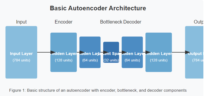
Let’s break down the structure of a basic autoencoder:

1. Input Layer: Receives your original data (e.g., images, text vectors, sensor readings)
2. Encoder Layers: A series of progressively smaller neural network layers
3. Latent Space (Bottleneck): The compressed representation of your data
4. Decoder Layers: A series of progressively larger neural network layers
5. Output Layer: Attempts to reconstruct the original input

During training, the autoencoder learns to minimize the difference between its input and output. In other words, it tries to create a faithful reconstruction while passing through the information bottleneck. Through this process, it discovers the most important features of your data.

Types of Autoencoders for Different Needs

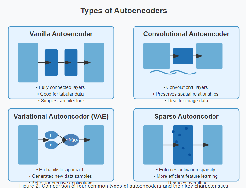
Autoencoders come in several flavors, each with specific strengths:

Vanilla Autoencoders

The simplest form, using fully connected layers. These work well for tabular data but may struggle with complex structures.

Convolutional Autoencoders

Specially designed for image data, these use convolutional layers to preserve spatial relationships. Furthermore, they’re excellent for image compression and denoising tasks.

Variational Autoencoders (VAEs)

These introduce probabilistic elements, representing the latent space as probability distributions rather than fixed points. Consequently, VAEs excel at generative tasks like creating new, realistic data samples.

Sparse Autoencoders

By adding constraints that encourage sparsity in the hidden layers, these autoencoders learn more efficient representations. As a result, they can often extract more meaningful features.

Practical Applications of Autoencoders

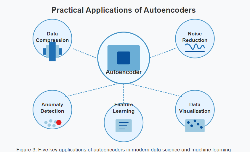
The versatility of autoencoders opens doors to numerous applications:

1. Data Compression: Reduce storage requirements while preserving essential information
2. Noise Reduction: Clean up noisy data by learning to reconstruct clean signals
3. Anomaly Detection: Identify unusual patterns that don’t fit the learned representations
4. Feature Learning: Discover meaningful features automatically from unlabeled data
5. Data Visualization: Project high-dimensional data to 2D or 3D for visualization

For instance, in healthcare, autoencoders help analyze complex patient data by reducing noise in medical images. Meanwhile, in cybersecurity, they detect unusual network traffic patterns that might indicate attacks.

Implementing Your First Autoencoder with Python

Let’s get our hands dirty with a practical example. We’ll build a simple autoencoder for dimensionality reduction using TensorFlow and Keras:

import numpy as np
import tensorflow as tf
from tensorflow.keras.layers import Input, Dense
from tensorflow.keras.models import Model
from tensorflow.keras.datasets import mnist
import matplotlib.pyplot as plt

# Load and preprocess data
(x_train, _), (x_test, _) = mnist.load_data()
x_train = x_train.astype('float32') / 255.
x_test = x_test.astype('float32') / 255.
x_train = x_train.reshape((len(x_train), np.prod(x_train.shape[1:])))
x_test = x_test.reshape((len(x_test), np.prod(x_test.shape[1:])))

# Set encoding dimension (our bottleneck size)
encoding_dim = 32  # 32 floats -> compression factor of 24.5 (784/32)

# Build the autoencoder model
# First, we define our input layer
input_img = Input(shape=(784,))

# The encoder part
encoded = Dense(128, activation='relu')(input_img)
encoded = Dense(64, activation='relu')(encoded)
encoded = Dense(encoding_dim, activation='relu')(encoded)

# The decoder part
decoded = Dense(64, activation='relu')(encoded)
decoded = Dense(128, activation='relu')(decoded)
decoded = Dense(784, activation='sigmoid')(decoded)

# Create the autoencoder model
autoencoder = Model(input_img, decoded)

# Also create a separate encoder model
encoder = Model(input_img, encoded)

# Compile the autoencoder
autoencoder.compile(optimizer='adam', loss='binary_crossentropy')

# Train the autoencoder
history = autoencoder.fit(
    x_train, x_train,
    epochs=20,
    batch_size=256,
    shuffle=True,
    validation_data=(x_test, x_test)
)

# Encode and decode some test images
encoded_imgs = encoder.predict(x_test)
decoded_imgs = autoencoder.predict(x_test)

# Visualize the results
n = 10  # Number of images to display
plt.figure(figsize=(20, 4))
for i in range(n):
    # Original images
    ax = plt.subplot(2, n, i + 1)
    plt.imshow(x_test[i].reshape(28, 28))
    plt.gray()
    ax.get_xaxis().set_visible(False)
    ax.get_yaxis().set_visible(False)
    
    # Reconstructed images
    ax = plt.subplot(2, n, i + 1 + n)
    plt.imshow(decoded_imgs[i].reshape(28, 28))
    plt.gray()
    ax.get_xaxis().set_visible(False)
    ax.get_yaxis().set_visible(False)
plt.show()

# Now let's visualize the latent space (2D projection using PCA)
from sklearn.decomposition import PCA

pca = PCA(n_components=2)
encoded_imgs_2d = pca.fit_transform(encoded_imgs)

plt.figure(figsize=(12, 10))
plt.scatter(encoded_imgs_2d[:, 0], encoded_imgs_2d[:, 1], c=y_test)
plt.colorbar()
plt.title('Visualization of the encoded representations')
plt.show()

In this example, we’ve built an autoencoder that compresses MNIST handwritten digit images from 784 dimensions (28×28 pixels) down to just 32 dimensions. Then, it reconstructs the images from this compressed representation.

Fine-Tuning Your Autoencoder for Better Results

Getting the best performance from your autoencoder requires careful tuning. Here are some key considerations:

Finding the Right Bottleneck Size

Too large, and your autoencoder won’t learn meaningful compression. Too small, and it might lose important information. Therefore, experiment with different sizes for your specific data.

Choosing Appropriate Activation Functions

For the hidden layers, ReLU often works well. However, for the output layer, choose based on your data range:

• Sigmoid for data normalized to [0,1]
• Tanh for data normalized to [-1,1]
• Linear for unbounded data

Selecting the Right Loss Function

The loss function should match your data type:

• Mean Squared Error for continuous data
• Binary Cross-Entropy for binary or normalized data
• Categorical Cross-Entropy for categorical data

Common Challenges and How to Overcome Them

Even experienced practitioners face challenges with autoencoders. Let’s look at some common issues:

Overfitting

When your autoencoder memorizes the training data instead of learning meaningful representations, it’s overfitting. To combat this, try:

• Adding dropout layers
• Using regularization
• Implementing early stopping

Vanishing Gradients

Deep autoencoders can suffer from vanishing gradients. In this case, consider:

• Using batch normalization
• Implementing skip connections
• Trying different activation functions

Balancing Reconstruction vs. Compression

Finding the sweet spot between reconstruction quality and compression rate is tricky. Hence, experiment with different architectures and loss function weightings to find the right balance for your application.

Beyond Basic Autoencoders: Advanced Techniques

Once you’ve mastered the basics, explore these advanced techniques:

Transfer Learning with Autoencoders

Pre-train your autoencoder on a large dataset, then fine-tune it for your specific task with limited data.

Adversarial Autoencoders

Combine autoencoders with adversarial training to create more realistic reconstructions and better latent representations.

Sequence Autoencoders

Designed for sequential data like text or time series, these use recurrent layers (LSTM or GRU) instead of dense layers.

Conclusion: Harnessing the Power of Autoencoders

Autoencoders represent a fascinating intersection of neural networks and dimensionality reduction. Their ability to learn complex data representations makes them invaluable tools in the modern data scientist’s toolkit.

By now, you should have a solid understanding of how autoencoders work and how to implement them for your own projects. Furthermore, you’ve seen how they can transform high-dimensional data into meaningful, compact representations.

Remember, mastering autoencoders takes practice. Start with simple implementations, then gradually explore more complex architectures as your confidence grows. Above all, experiment with your own data to discover the unique insights autoencoders can reveal.

What dimensionality reduction challenge will you tackle first with autoencoders? The possibilities are endless!

References

1. TensorFlow Autoencoder Guide
2. Keras Autoencoders Example
3. Original Autoencoder Research Paper
4. Ultimate Guide to Activation Functions for Neural Networks
5. Neural Networks Made Easy – Start Coding Now!

Did you find this introduction to autoencoders helpful? Share your thoughts or questions in the comments below!