Linear regression is a fundamental statistical technique used for predictive modelling. It allows us to understand the relationship between a dependent variable (target) and one or more independent variables (predictors). There are several types of linear regression, each catering to different data complexities and patterns.

Despite all the buzz around deep learning and complex AI models, linear regression remains a cornerstone of data science. In my experience working with startups and enterprise companies, I’ve found that understanding linear regression is crucial for:

– Predictive analytics

– Statistical modeling

– Machine learning foundations

– Data-driven decision making

– Business forecasting

Let’s dive into the different types and see how they can solve real-world problems.

1. Simple Linear Regression:

Remember in school when we learned about plotting points on a graph? Simple linear regression is basically that, but with superpowers!

The Math Behind It (Don’t Run Away Just Yet!)

Y=β0+β1X+ϵ

Where:

• Y is the dependent variable
• β0 is the y-intercept
• β1 is the slope of the line
• X is the independent variable
• ϵ is the error term

When to Use:

Use simple linear regression when you have only one independent variable and want to understand or predict the relationship between it and the dependent variable.

Real-World Application

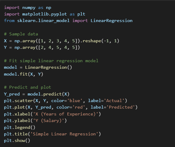
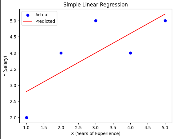
Suppose you want to predict the salary of employees based on their years of experience. Here, represents years of experience, and represents salary.

Below is a simple visualization of a dataset for Simple Linear Regression.

“`python

Here’s how I typically implement it in Python

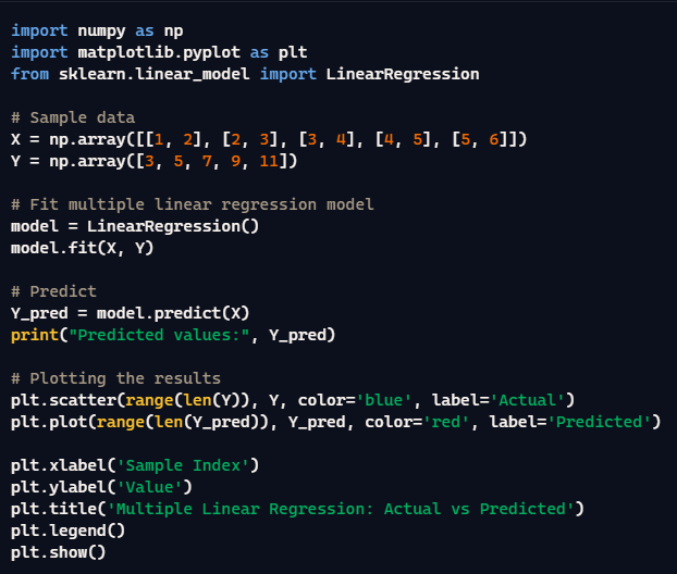
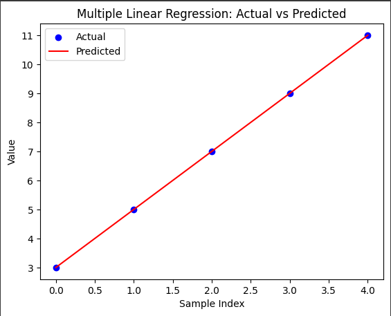
2. Multiple Linear Regression: When Life Gets Complicated

Multiple linear regression models the relationship between a dependent variable and two or more independent variables.

In reality, house prices depend on more than just square footage. This is where multiple linear regression shines. I use this all the time when dealing with complex predictions.

The Secret Sauce (Mathematical Intuition)

Your prediction now looks like:

y = β₀ + β₁x₁ + β₂ x₂ + … + βₙxₙ + ε

Where:

• y is the dependent variable
• β₀ is the y-intercept
• β₁ is the slope of the line
• x₁, x₂.. xₙ are the independent variable
• ϵ is the error term

The optimal coefficients are obtained by minimizing the sum of squared errors (SSE)

When to Use:

Use multiple linear regression when you have more than one independent variable, and you want to explore how each feature affects the dependent variable.

Think of it as juggling multiple factors at once – location, number of bedrooms, age of the house, etc.

Real-World Application

Predicting house prices based on features like area, number of bedrooms, and location.

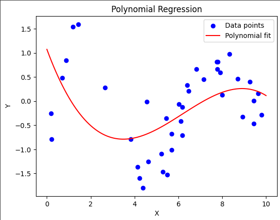
## 3. Polynomial Regression: Handling Curves Like a Pro

Sometimes, relationships aren’t straight lines. I learned this the hard way when analyzing customer satisfaction scores! Polynomial regression saved the day by allowing for curved relationships.

Have you ever tried to fit a straight line to data points, only to find that the relationship between the variables is more complex? That’s where polynomial regression comes in handy! 🌟

Mathematical Intuition

 

Where d is called the degree of polynomial

When to Use It

– Product pricing optimization

– Population growth modeling

– Environmental data analysis

– Customer behaviour prediction

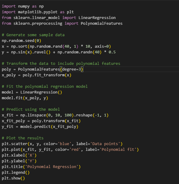
Python Code for Polynomial Regression

Let’s dive into some Python code to see polynomial regression in action. We’ll use the scikit-learn library to perform polynomial regression and visualize the results.

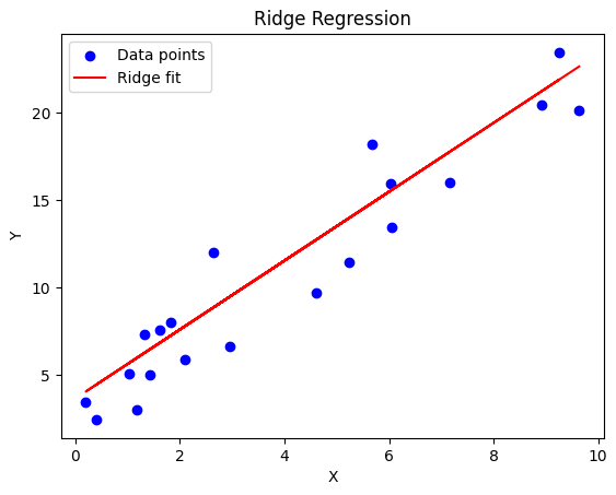
4. Ridge Regression (L2 Regularization): Taming Wild Data

Remember the first time you dealt with multicollinearity? I sure do! Ridge regression is like having a safety net for your model.

Ever felt overwhelmed by wild data that just won’t fit neatly into your models? Ridge regression is also called Tikhonov Regularization which deals with multicollinearity.🛡️

Ridge Regression is a type of linear regression that includes a regularization term, which helps to reduce the complexity of the model. Unlike ordinary least squares, which minimizes the sum of squared errors (SSE), Ridge adds a penalty term to the loss function. This penalty discourages large coefficients in the model.

The Math (Made Simple)

We add a penalty term to prevent coefficients from getting too large:

min(||y – Xβ||² + α||β||²)

||y – Xβ||²: This term represents the sum of squared residuals, which is the difference between the observed values (y) and the predicted values (Xβ). In other words, it’s the error term that we want to minimize in ordinary least squares regression.

α||β||²: This is the regularization term, where (α) is the regularization parameter and (|β||²) is the sum of the squares of the coefficients. This term penalizes large coefficients, helping to prevent overfitting.

By minimizing the sum of these two terms, Ridge regression balances the fit of the model (how well it predicts the data) with the complexity of the model (how large the coefficients are). The regularization parameter (α) controls the trade-off between these two aspects. A larger (α) place more emphasis on shrinking the coefficients, while a smaller (α) place more emphasis on fitting the data closely.

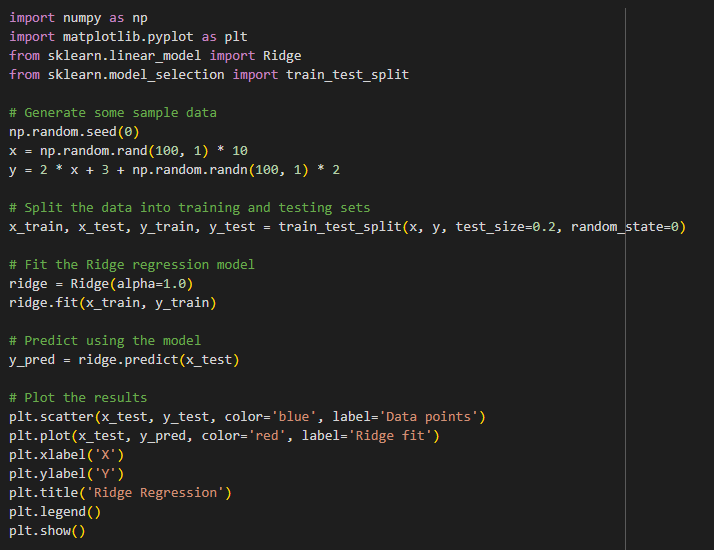
Python Code for Ridge Regression

5. Lasso Regression: Feature Selection on Autopilot

One of my favourite techniques for dealing with feature selection. It’s like having an automated feature selector built into your regression!

Ever wished your model could automatically select the most important features? Lasso regression might be just what you need! 🌟

Pro Tips from Experience

– Start with a range of alpha values

– Use cross-validation to find the optimal parameter

– Monitor which features get eliminated

Mathematical Intuition

minimize: ||Y – Xβ||² + λ||β||₁

Where:

• ||Y – Xβ||² is the ordinary least squares (OLS) term:
  • Y is the vector of target variables
  • X is the matrix of features
  • β is the vector of coefficients
  • ||·||² represents the L2 norm (sum of squared residuals)
• λ||β||₁ is the regularization term:
  • λ (lambda) is the regularization parameter (λ ≥ 0)
  • ||β||₁ represents the L1 norm of the coefficient vector (sum of absolute values)

 

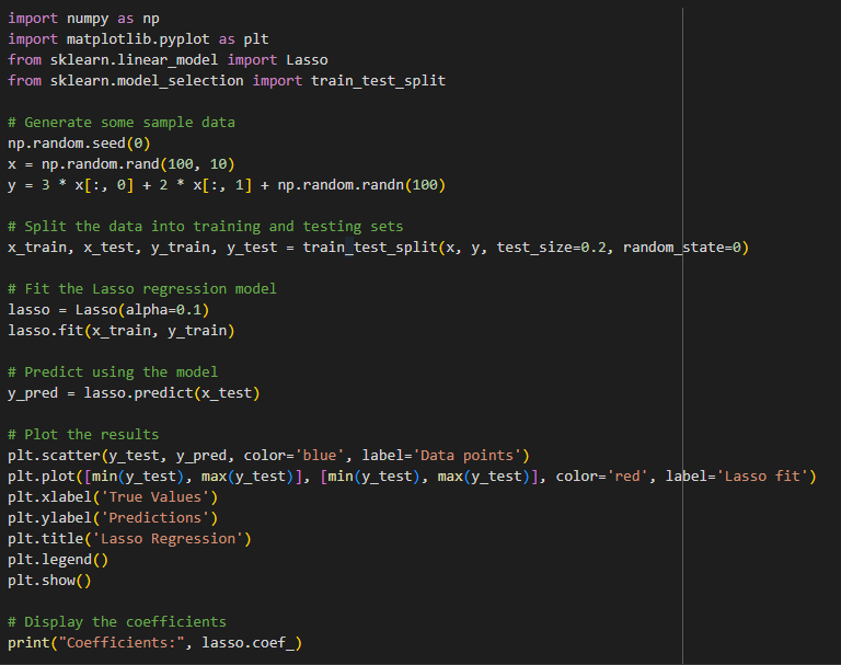
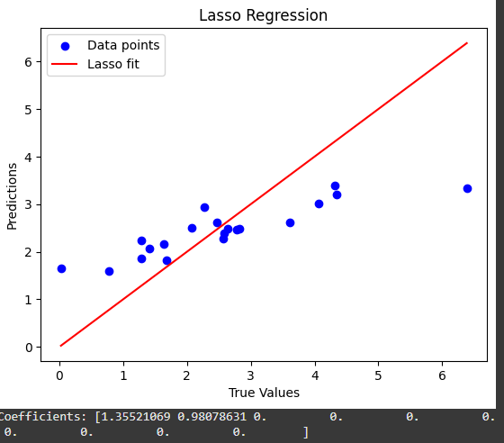
Python Code for Lasso Regression

6. Elastic Net: The Best of Both Worlds

Think of Elastic Net as the Swiss Army knife of regression techniques. It combines the powers of Ridge and Lasso regression.

Struggling to choose between Ridge and Lasso regression? Why not get the best of both worlds with Elastic Net! 🌟

Mathematical Intuition

minimize: ||Y – Xβ||² + λ₁||β||₁ + λ₂||β||²

Where:

• ||Y – Xβ||² is the OLS term
• λ₁||β||₁ is the L1 (Lasso) penalty
• λ₂||β||² is the L2 (Ridge) penalty
• λ₁ and λ₂ are regularization parameters

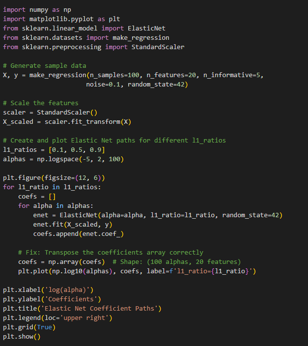
Python Code for Elastic Net Regression

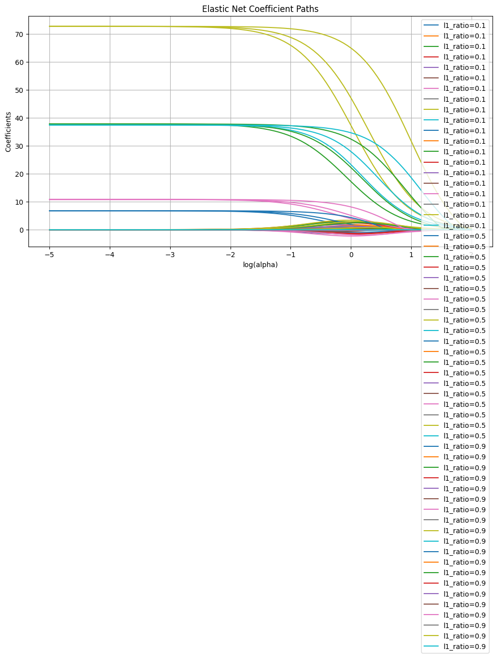
The resulting plot shows coefficient paths where:

• Horizontal axis: regularization strength (log scale)
• Vertical axis: coefficient values
• Different lines: how each feature’s importance changes
• Different colors: different l1_ratio values

——————————————————————————————–

Common Pitfalls and How to Avoid Them

After years of teaching and applying these concepts, here are some tips:

1. Data Preprocessing is Key

– Always check for outliers

– Scale your features when needed

– Handle missing values appropriately

2. Model Validation

– Don’t just rely on R-squared

– Use k-fold cross-validation

– Check residual plots

3. Feature Engineering

– Create interaction terms when it makes sense

– Consider domain knowledge

– Don’t blindly include all variables

Tools and Technologies

Here’s my go-to toolkit for regression analysis:

– Python’s scikit-learn

– statsmodels for detailed statistical analysis

– Pandas for data manipulation

– Seaborn and Matplotlib for visualization

Future Trends in Regression Analysis

As we move through 2025, I’m seeing some exciting developments:

– AutoML tools for automated regression analysis

– Integration with big data frameworks

– Enhanced visualization techniques

– Real-time regression analysis

Conclusion

Linear regression might seem basic, but it’s like the foundation of a house – you need it to be rock solid. I hope this guide helps you understand not just the how, but the why of regression analysis.